I have to tell you about the Kalman filter, because what it does is pretty damn amazing.
Surprisingly few software engineers and scientists seem to know about it, and that makes me sad because it is such a general and powerful tool for combining information in the presence of uncertainty. At times its ability to extract accurate information seems almost magical— and if it sounds like I’m talking this up too much, then take a look at this previously posted video where I demonstrate a Kalman filter figuring out the orientation of a free-floating body by looking at its velocity. Totally neat!
What is it?
You can use a Kalman filter in any place where you have uncertain information about some dynamic system, and you can make an educated guess about what the system is going to do next. Even if messy reality comes along and interferes with the clean motion you guessed about, the Kalman filter will often do a very good job of figuring out what actually happened. And it can take advantage of correlations between crazy phenomena that you maybe wouldn’t have thought to exploit!
Kalman filters are ideal for systems which are continuously changing. They have the advantage that they are light on memory (they don’t need to keep any history other than the previous state), and they are very fast, making them well suited for real time problems and embedded systems.
The math for implementing the Kalman filter appears pretty scary and opaque in most places you find on Google. That’s a bad state of affairs, because the Kalman filter is actually super simple and easy to understand if you look at it in the right way. Thus it makes a great article topic, and I will attempt to illuminate it with lots of clear, pretty pictures and colors. The prerequisites are simple; all you need is a basic understanding of probability and matrices.
I’ll start with a loose example of the kind of thing a Kalman filter can solve, but if you want to get right to the shiny pictures and math, feel free to jump ahead.
What can we do with a Kalman filter?
Let’s make a toy example: You’ve built a little robot that can wander around in the woods, and the robot needs to know exactly where it is so that it can navigate.

We’ll say our robot has a state \( \vec{x_k} \), which is just a position and a velocity:
\(\vec{x_k} = (\vec{p}, \vec{v})\)
Note that the state is just a list of numbers about the underlying configuration of your system; it could be anything. In our example it’s position and velocity, but it could be data about the amount of fluid in a tank, the temperature of a car engine, the position of a user’s finger on a touchpad, or any number of things you need to keep track of.
Our robot also has a GPS sensor, which is accurate to about 10 meters, which is good, but it needs to know its location more precisely than 10 meters. There are lots of gullies and cliffs in these woods, and if the robot is wrong by more than a few feet, it could fall off a cliff. So GPS by itself is not good enough.
We might also know something about how the robot moves: It knows the commands sent to the wheel motors, and its knows that if it’s headed in one direction and nothing interferes, at the next instant it will likely be further along that same direction. But of course it doesn’t know everything about its motion: It might be buffeted by the wind, the wheels might slip a little bit, or roll over bumpy terrain; so the amount the wheels have turned might not exactly represent how far the robot has actually traveled, and the prediction won’t be perfect.
The GPS sensor tells us something about the state, but only indirectly, and with some uncertainty or inaccuracy. Our prediction tells us something about how the robot is moving, but only indirectly, and with some uncertainty or inaccuracy.
But if we use all the information available to us, can we get a better answer than either estimate would give us by itself? Of course the answer is yes, and that’s what a Kalman filter is for.
How a Kalman filter sees your problem
Let’s look at the landscape we’re trying to interpret. We’ll continue with a simple state having only position and velocity. $$
\vec{x} = \begin{bmatrix}
p\\
v
\end{bmatrix}$$
We don’t know what the actual position and velocity are; there are a whole range of possible combinations of position and velocity that might be true, but some of them are more likely than others:
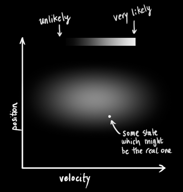
The Kalman filter assumes that both variables (postion and velocity, in our case) are random and Gaussian distributed. Each variable has a mean value \(\mu\), which is the center of the random distribution (and its most likely state), and a variance \(\sigma^2\), which is the uncertainty:
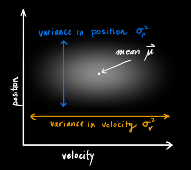
In the above picture, position and velocity are uncorrelated, which means that the state of one variable tells you nothing about what the other might be.
The example below shows something more interesting: Position and velocity are correlated. The likelihood of observing a particular position depends on what velocity you have:
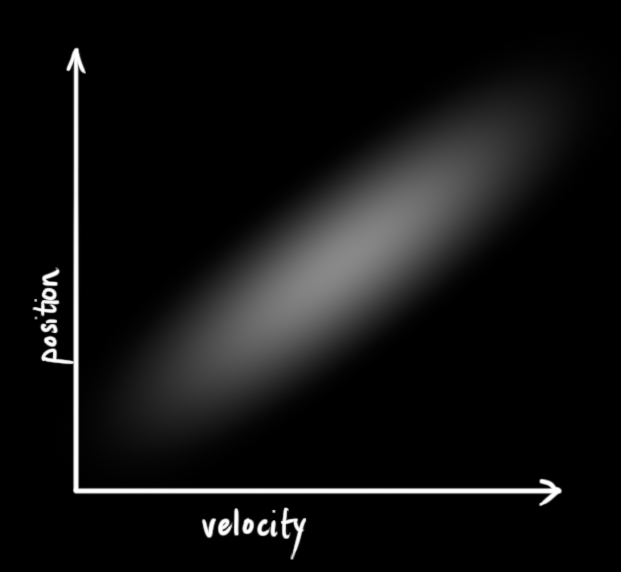 This kind of situation might arise if, for example, we are estimating a new position based on an old one. If our velocity was high, we probably moved farther, so our position will be more distant. If we’re moving slowly, we didn’t get as far.
This kind of relationship is really important to keep track of, because it gives us more information: One measurement tells us something about what the others could be. And that’s the goal of the Kalman filter, we want to squeeze as much information from our uncertain measurements as we possibly can!
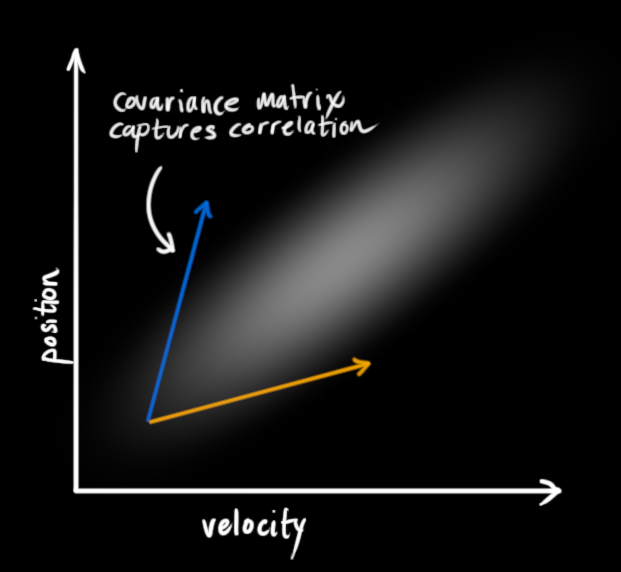
This correlation is captured by something called a covariance matrix. In short, each element of the matrix \(\Sigma_{ij}\) is the degree of correlation between the ith state variable and the jth state variable. (You might be able to guess that the covariance matrix is symmetric, which means that it doesn’t matter if you swap i and j). Covariance matrices are often labelled “\(\mathbf{\Sigma}\)”, so we call their elements “\(\Sigma_{ij}\)”.
Describing the problem with matrices
We’re modeling our knowledge about the state as a Gaussian blob, so we need two pieces of information at time \(k\): We’ll call our best estimate \(\mathbf{\hat{x}_k}\) (the mean, elsewhere named \(\mu\) ), and its covariance matrix \(\mathbf{P_k}\). $$
\begin{equation} \label{eq:statevars}
\begin{aligned}
\mathbf{\hat{x}}_k &= \begin{bmatrix}
\text{position}\\
\text{velocity}
\end{bmatrix}\\
\mathbf{P}_k &=
\begin{bmatrix}
\Sigma_{pp} & \Sigma_{pv} \\
\Sigma_{vp} & \Sigma_{vv} \\
\end{bmatrix}
\end{aligned}
\end{equation}
$$
(Of course we are using only position and velocity here, but it’s useful to remember that the state can contain any number of variables, and represent anything you want).
Next, we need some way to look at the current state (at time k-1) and predict the next state at time k. Remember, we don’t know which state is the “real” one, but our prediction function doesn’t care. It just works on all of them, and gives us a new distribution:
 We can represent this prediction step with a matrix, \(\mathbf{F_k}\):
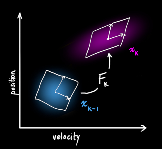 It takes every point in our original estimate and moves it to a new predicted location, which is where the system would move if that original estimate was the right one.
Let’s apply this. How would we use a matrix to predict the position and velocity at the next moment in the future? We’ll use a really basic kinematic formula:$$
\begin{split}
\color{deeppink}{p_k} &= \color{royalblue}{p_{k-1}} + \Delta t &\color{royalblue}{v_{k-1}} \\
\color{deeppink}{v_k} &= &\color{royalblue}{v_{k-1}}
\end{split}
$$ In other words: $$
\begin{align}
\color{deeppink}{\mathbf{\hat{x}}_k} &= \begin{bmatrix}
1 & \Delta t \\
0 & 1
\end{bmatrix} \color{royalblue}{\mathbf{\hat{x}}_{k-1}} \\
&= \mathbf{F}_k \color{royalblue}{\mathbf{\hat{x}}_{k-1}} \label{statevars}
\end{align}
$$
We now have a prediction matrix which gives us our next state, but we still don’t know how to update the covariance matrix.
This is where we need another formula. If we multiply every point in a distribution by a matrix \(\color{firebrick}{\mathbf{A}}\), then what happens to its covariance matrix \(\Sigma\)?
Well, it’s easy. I’ll just give you the identity:$$
\begin{equation}
\begin{split}
Cov(x) &= \Sigma\\
Cov(\color{firebrick}{\mathbf{A}}x) &= \color{firebrick}{\mathbf{A}} \Sigma \color{firebrick}{\mathbf{A}}^T
\end{split} \label{covident}
\end{equation}
$$
So combining \(\eqref{covident}\) with equation \(\eqref{statevars}\):$$
\begin{equation}
\begin{split}
\color{deeppink}{\mathbf{\hat{x}}_k} &= \mathbf{F}_k \color{royalblue}{\mathbf{\hat{x}}_{k-1}} \\
\color{deeppink}{\mathbf{P}_k} &= \mathbf{F_k} \color{royalblue}{\mathbf{P}_{k-1}} \mathbf{F}_k^T
\end{split}
\end{equation}
$$
External influence
We haven’t captured everything, though. There might be some changes that aren’t related to the state itself— the outside world could be affecting the system.
For example, if the state models the motion of a train, the train operator might push on the throttle, causing the train to accelerate. Similarly, in our robot example, the navigation software might issue a command to turn the wheels or stop. If we know this additional information about what’s going on in the world, we could stuff it into a vector called \(\color{darkorange}{\vec{\mathbf{u}_k}}\), do something with it, and add it to our prediction as a correction.
Let’s say we know the expected acceleration \(\color{darkorange}{a}\) due to the throttle setting or control commands. From basic kinematics we get: $$
\begin{split}
\color{deeppink}{p_k} &= \color{royalblue}{p_{k-1}} + {\Delta t} &\color{royalblue}{v_{k-1}} + &\frac{1}{2} \color{darkorange}{a} {\Delta t}^2 \\
\color{deeppink}{v_k} &= &\color{royalblue}{v_{k-1}} + & \color{darkorange}{a} {\Delta t}
\end{split}
$$ In matrix form: $$
\begin{equation}
\begin{split}
\color{deeppink}{\mathbf{\hat{x}}_k} &= \mathbf{F}_k \color{royalblue}{\mathbf{\hat{x}}_{k-1}} + \begin{bmatrix}
\frac{\Delta t^2}{2} \\
\Delta t
\end{bmatrix} \color{darkorange}{a} \\
&= \mathbf{F}_k \color{royalblue}{\mathbf{\hat{x}}_{k-1}} + \mathbf{B}_k \color{darkorange}{\vec{\mathbf{u}_k}}
\end{split}
\end{equation}
$$
\(\mathbf{B}_k\) is called the control matrix and \(\color{darkorange}{\vec{\mathbf{u}_k}}\) the control vector. (For very simple systems with no external influence, you could omit these).
Let’s add one more detail. What happens if our prediction is not a 100% accurate model of what’s actually going on?
External uncertainty
Everything is fine if the state evolves based on its own properties. Everything is still fine if the state evolves based on external forces, so long as we know what those external forces are.
But what about forces that we don’t know about? If we’re tracking a quadcopter, for example, it could be buffeted around by wind. If we’re tracking a wheeled robot, the wheels could slip, or bumps on the ground could slow it down. We can’t keep track of these things, and if any of this happens, our prediction could be off because we didn’t account for those extra forces.
We can model the uncertainty associated with the “world” (i.e. things we aren’t keeping track of) by adding some new uncertainty after every prediction step:
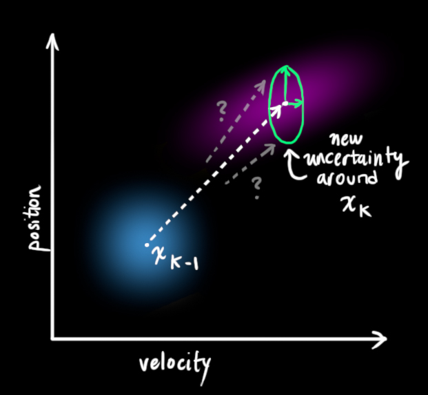
Every state in our original estimate could have moved to a range of states. Because we like Gaussian blobs so much, we’ll say that each point in \(\color{royalblue}{\mathbf{\hat{x}}_{k-1}}\) is moved to somewhere inside a Gaussian blob with covariance \(\color{mediumaquamarine}{\mathbf{Q}_k}\). Another way to say this is that we are treating the untracked influences as noise with covariance \(\color{mediumaquamarine}{\mathbf{Q}_k}\).
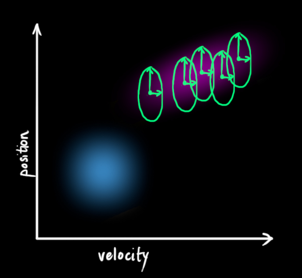 This produces a new Gaussian blob, with a different covariance (but the same mean):
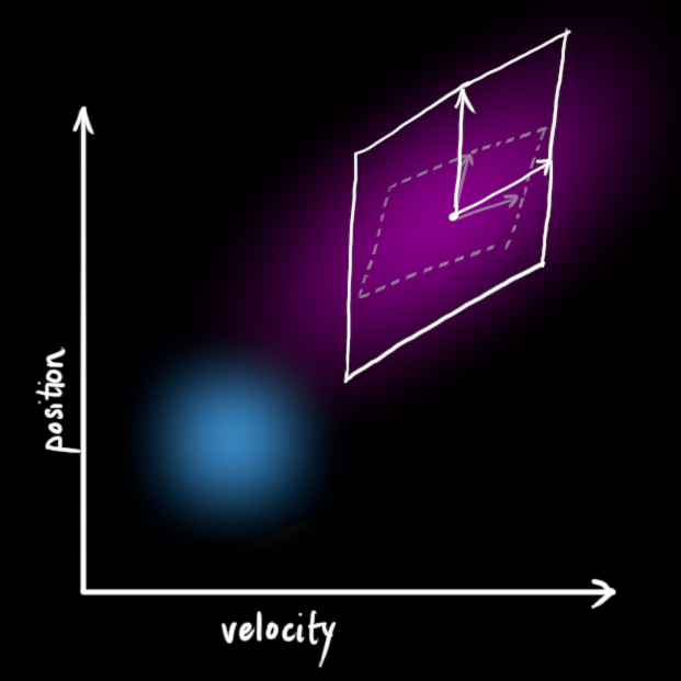
We get the expanded covariance by simply adding \({\color{mediumaquamarine}{\mathbf{Q}_k}}\), giving our complete expression for the prediction step: $$
\begin{equation}
\begin{split}
\color{deeppink}{\mathbf{\hat{x}}_k} &= \mathbf{F}_k \color{royalblue}{\mathbf{\hat{x}}_{k-1}} + \mathbf{B}_k \color{darkorange}{\vec{\mathbf{u}_k}} \\
\color{deeppink}{\mathbf{P}_k} &= \mathbf{F_k} \color{royalblue}{\mathbf{P}_{k-1}} \mathbf{F}_k^T + \color{mediumaquamarine}{\mathbf{Q}_k}
\end{split}
\label{kalpredictfull}
\end{equation}
$$
In other words, the new best estimate is a prediction made from previous best estimate, plus a correction for known external influences.
And the new uncertainty is predicted from the old uncertainty, with some additional uncertainty from the environment.
All right, so that’s easy enough. We have a fuzzy estimate of where our system might be, given by \(\color{deeppink}{\mathbf{\hat{x}}_k}\) and \(\color{deeppink}{\mathbf{P}_k}\). What happens when we get some data from our sensors?
Refining the estimate with measurements
We might have several sensors which give us information about the state of our system. For the time being it doesn’t matter what they measure; perhaps one reads position and the other reads velocity. Each sensor tells us something indirect about the state— in other words, the sensors operate on a state and produce a set of readings.
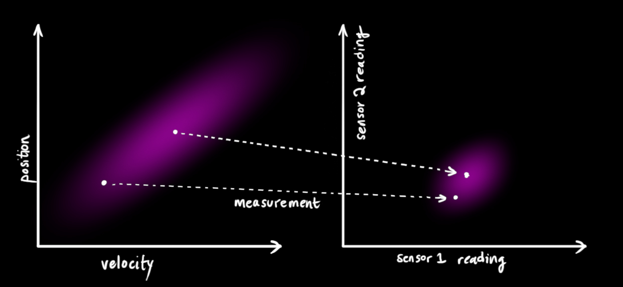 Notice that the units and scale of the reading might not be the same as the units and scale of the state we’re keeping track of. You might be able to guess where this is going: We’ll model the sensors with a matrix, \(\mathbf{H}_k\).
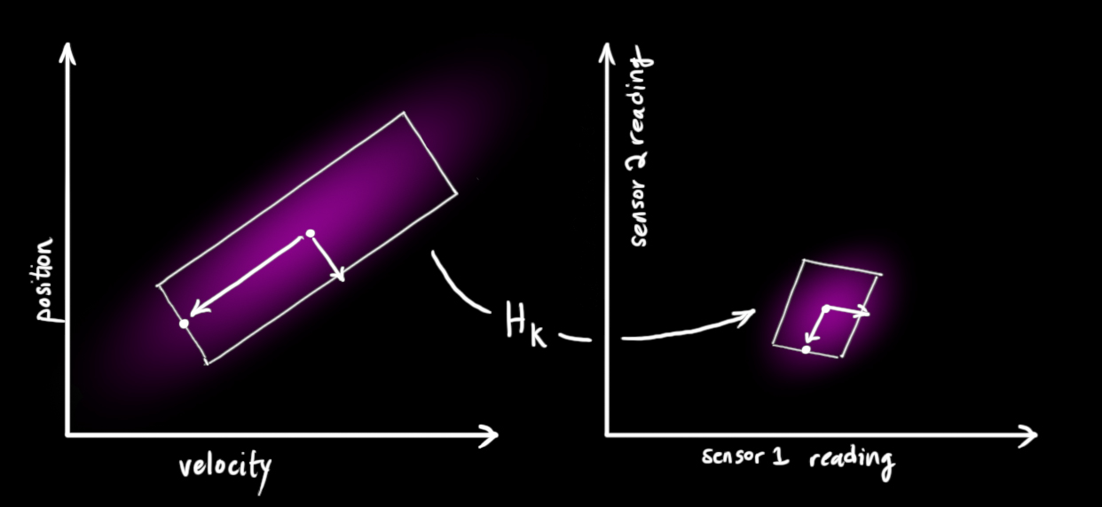
We can figure out the distribution of sensor readings we’d expect to see in the usual way: $$
\begin{equation}
\begin{aligned}
\vec{\mu}_{\text{expected}} &= \mathbf{H}_k \color{deeppink}{\mathbf{\hat{x}}_k} \\
\mathbf{\Sigma}_{\text{expected}} &= \mathbf{H}_k \color{deeppink}{\mathbf{P}_k} \mathbf{H}_k^T
\end{aligned}
\end{equation}
$$
One thing that Kalman filters are great for is dealing with sensor noise. In other words, our sensors are at least somewhat unreliable, and every state in our original estimate might result in a range of sensor readings. 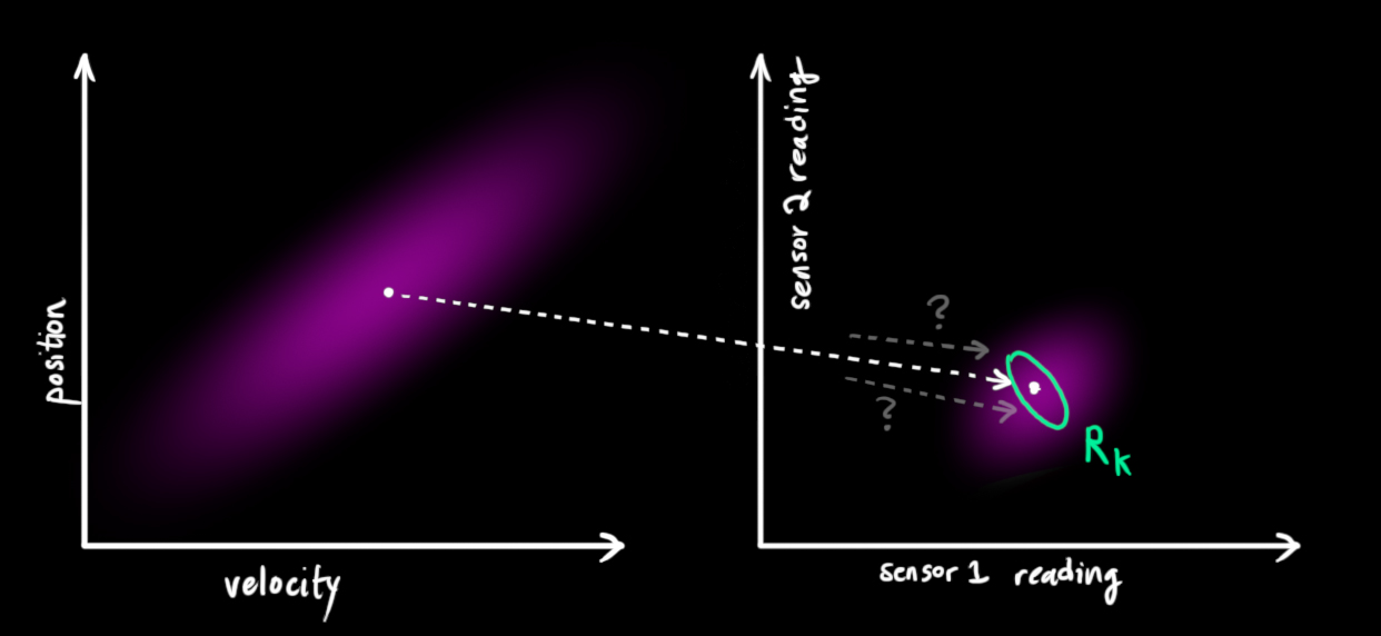
From each reading we observe, we might guess that our system was in a particular state. But because there is uncertainty, some states are more likely than others to have have produced the reading we saw: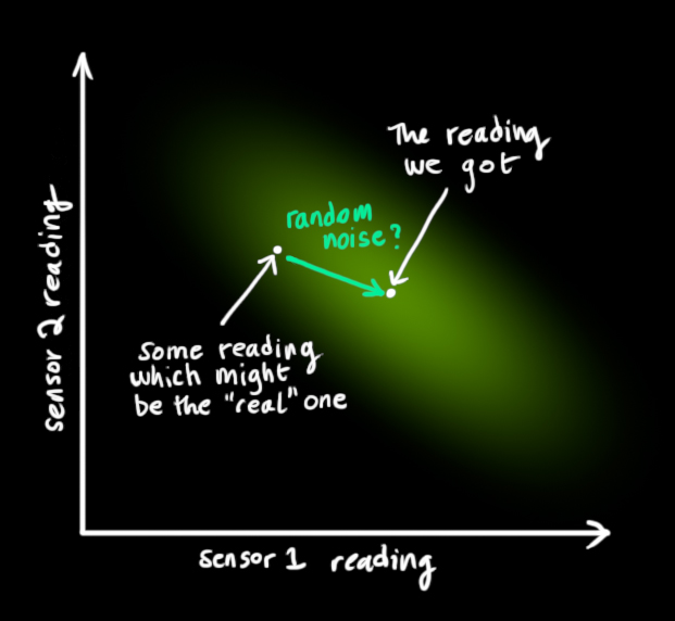
We’ll call the covariance of this uncertainty (i.e. of the sensor noise) \(\color{mediumaquamarine}{\mathbf{R}_k}\). The distribution has a mean equal to the reading we observed, which we’ll call \(\color{yellowgreen}{\vec{\mathbf{z}_k}}\).
So now we have two Gaussian blobs: One surrounding the mean of our transformed prediction, and one surrounding the actual sensor reading we got.
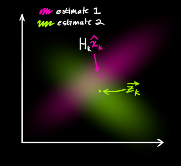
We must try to reconcile our guess about the readings we’d see based on the predicted state (pink) with a different guess based on our sensor readings (green) that we actually observed.
So what’s our new most likely state? For any possible reading \((z_1,z_2)\), we have two associated probabilities: (1) The probability that our sensor reading \(\color{yellowgreen}{\vec{\mathbf{z}_k}}\) is a (mis-)measurement of \((z_1,z_2)\), and (2) the probability that our previous estimate thinks \((z_1,z_2)\) is the reading we should see.
If we have two probabilities and we want to know the chance that both are true, we just multiply them together. So, we take the two Gaussian blobs and multiply them:
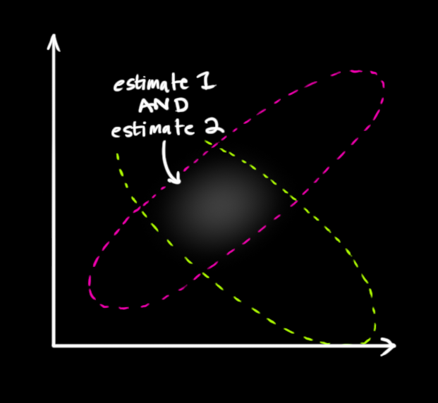
What we’re left with is the overlap, the region where both blobs are bright/likely. And it’s a lot more precise than either of our previous estimates. The mean of this distribution is the configuration for which both estimates are most likely, and is therefore the best guess of the true configuration given all the information we have.
Hmm. This looks like another Gaussian blob.
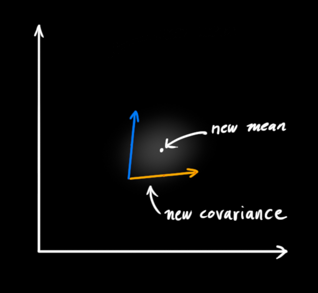
As it turns out, when you multiply two Gaussian blobs with separate means and covariance matrices, you get a new Gaussian blob with its own mean and covariance matrix! Maybe you can see where this is going: There’s got to be a formula to get those new parameters from the old ones!
Combining Gaussians
Let’s find that formula. It’s easiest to look at this first in one dimension. A 1D Gaussian bell curve with variance \(\sigma^2\) and mean \(\mu\) is defined as: $$
\begin{equation} \label{gaussformula}
\mathcal{N}(x, \mu,\sigma) = \frac{1}{ \sigma \sqrt{ 2\pi } } e^{ -\frac{ (x – \mu)^2 }{ 2\sigma^2 } }
\end{equation}
$$
We want to know what happens when you multiply two Gaussian curves together. The blue curve below represents the (unnormalized) intersection of the two Gaussian populations:
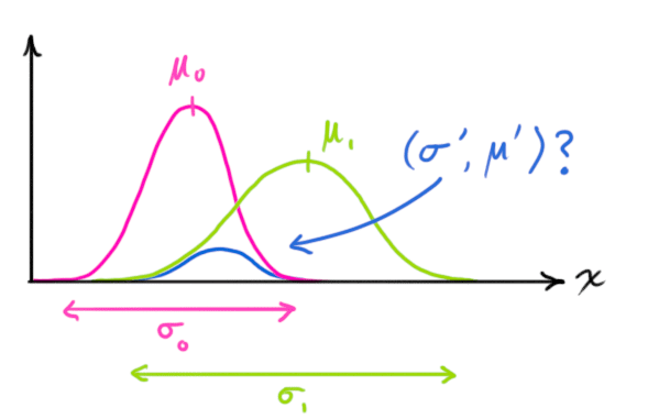
$$\begin{equation} \label{gaussequiv}
\mathcal{N}(x, \color{fuchsia}{\mu_0}, \color{deeppink}{\sigma_0}) \cdot \mathcal{N}(x, \color{yellowgreen}{\mu_1}, \color{mediumaquamarine}{\sigma_1}) \stackrel{?}{=} \mathcal{N}(x, \color{royalblue}{\mu’}, \color{mediumblue}{\sigma’})
\end{equation}$$
You can substitute equation \(\eqref{gaussformula}\) into equation \(\eqref{gaussequiv}\) and do some algebra (being careful to renormalize, so that the total probability is 1) to obtain: $$
\begin{equation} \label{fusionformula}
\begin{aligned}
\color{royalblue}{\mu’} &= \mu_0 + \frac{\sigma_0^2 (\mu_1 – \mu_0)} {\sigma_0^2 + \sigma_1^2}\\
\color{mediumblue}{\sigma’}^2 &= \sigma_0^2 – \frac{\sigma_0^4} {\sigma_0^2 + \sigma_1^2}
\end{aligned}
\end{equation}$$
We can simplify by factoring out a little piece and calling it \(\color{purple}{\mathbf{k}}\): $$
\begin{equation} \label{gainformula}
\color{purple}{\mathbf{k}} = \frac{\sigma_0^2}{\sigma_0^2 + \sigma_1^2}
\end{equation} $$ $$
\begin{equation}
\begin{split}
\color{royalblue}{\mu’} &= \mu_0 + &\color{purple}{\mathbf{k}} (\mu_1 – \mu_0)\\
\color{mediumblue}{\sigma’}^2 &= \sigma_0^2 – &\color{purple}{\mathbf{k}} \sigma_0^2
\end{split} \label{update}
\end{equation} $$
Take note of how you can take your previous estimate and add something to make a new estimate. And look at how simple that formula is!
But what about a matrix version? Well, let’s just re-write equations \(\eqref{gainformula}\) and \(\eqref{update}\) in matrix form. If \(\Sigma\) is the covariance matrix of a Gaussian blob, and \(\vec{\mu}\) its mean along each axis, then: $$
\begin{equation} \label{matrixgain}
\color{purple}{\mathbf{K}} = \Sigma_0 (\Sigma_0 + \Sigma_1)^{-1}
\end{equation} $$ $$
\begin{equation}
\begin{split}
\color{royalblue}{\vec{\mu}’} &= \vec{\mu_0} + &\color{purple}{\mathbf{K}} (\vec{\mu_1} – \vec{\mu_0})\\
\color{mediumblue}{\Sigma’} &= \Sigma_0 – &\color{purple}{\mathbf{K}} \Sigma_0
\end{split} \label{matrixupdate}
\end{equation}
$$
\(\color{purple}{\mathbf{K}}\) is a matrix called the Kalman gain, and we’ll use it in just a moment.
Easy! We’re almost finished!
Putting it all together
We have two distributions: The predicted measurement with \( (\color{fuchsia}{\mu_0}, \color{deeppink}{\Sigma_0}) = (\color{fuchsia}{\mathbf{H}_k \mathbf{\hat{x}}_k}, \color{deeppink}{\mathbf{H}_k \mathbf{P}_k \mathbf{H}_k^T}) \), and the observed measurement with \( (\color{yellowgreen}{\mu_1}, \color{mediumaquamarine}{\Sigma_1}) = (\color{yellowgreen}{\vec{\mathbf{z}_k}}, \color{mediumaquamarine}{\mathbf{R}_k})\). We can just plug these into equation \(\eqref{matrixupdate}\) to find their overlap: $$
\begin{equation}
\begin{aligned}
\mathbf{H}_k \color{royalblue}{\mathbf{\hat{x}}_k’} &= \color{fuchsia}{\mathbf{H}_k \mathbf{\hat{x}}_k} & + & \color{purple}{\mathbf{K}} ( \color{yellowgreen}{\vec{\mathbf{z}_k}} – \color{fuchsia}{\mathbf{H}_k \mathbf{\hat{x}}_k} ) \\
\mathbf{H}_k \color{royalblue}{\mathbf{P}_k’} \mathbf{H}_k^T &= \color{deeppink}{\mathbf{H}_k \mathbf{P}_k \mathbf{H}_k^T} & – & \color{purple}{\mathbf{K}} \color{deeppink}{\mathbf{H}_k \mathbf{P}_k \mathbf{H}_k^T}
\end{aligned} \label {kalunsimplified}
\end{equation}
$$ And from \(\eqref{matrixgain}\), the Kalman gain is: $$
\begin{equation} \label{eq:kalgainunsimplified}
\color{purple}{\mathbf{K}} = \color{deeppink}{\mathbf{H}_k \mathbf{P}_k \mathbf{H}_k^T} ( \color{deeppink}{\mathbf{H}_k \mathbf{P}_k \mathbf{H}_k^T} + \color{mediumaquamarine}{\mathbf{R}_k})^{-1}
\end{equation}
$$ We can knock an \(\mathbf{H}_k\) off the front of every term in \(\eqref{kalunsimplified}\) and \(\eqref{eq:kalgainunsimplified}\) (note that one is hiding inside \(\color{purple}{\mathbf{K}}\) ), and an \(\mathbf{H}_k^T\) off the end of all terms in the equation for \(\color{royalblue}{\mathbf{P}_k’}\). $$
\begin{equation}
\begin{split}
\color{royalblue}{\mathbf{\hat{x}}_k’} &= \color{fuchsia}{\mathbf{\hat{x}}_k} & + & \color{purple}{\mathbf{K}’} ( \color{yellowgreen}{\vec{\mathbf{z}_k}} – \color{fuchsia}{\mathbf{H}_k \mathbf{\hat{x}}_k} ) \\
\color{royalblue}{\mathbf{P}_k’} &= \color{deeppink}{\mathbf{P}_k} & – & \color{purple}{\mathbf{K}’} \color{deeppink}{\mathbf{H}_k \mathbf{P}_k}
\end{split}
\label{kalupdatefull}
\end{equation} $$ $$
\begin{equation}
\color{purple}{\mathbf{K}’} = \color{deeppink}{\mathbf{P}_k \mathbf{H}_k^T} ( \color{deeppink}{\mathbf{H}_k \mathbf{P}_k \mathbf{H}_k^T} + \color{mediumaquamarine}{\mathbf{R}_k})^{-1}
\label{kalgainfull}
\end{equation}
$$ …giving us the complete equations for the update step.
And that’s it! \(\color{royalblue}{\mathbf{\hat{x}}_k’}\) is our new best estimate, and we can go on and feed it (along with \( \color{royalblue}{\mathbf{P}_k’} \) ) back into another round of predict or update as many times as we like.
Wrapping up
Of all the math above, all you need to implement are equations \(\eqref{kalpredictfull}, \eqref{kalupdatefull}\), and \(\eqref{kalgainfull}\). (Or if you forget those, you could re-derive everything from equations \(\eqref{covident}\) and \(\eqref{matrixupdate}\).)
This will allow you to model any linear system accurately. For nonlinear systems, we use the extended Kalman filter, which works by simply linearizing the predictions and measurements about their mean. (I may do a second write-up on the EKF in the future).
If I’ve done my job well, hopefully someone else out there will realize how cool these things are and come up with an unexpected new place to put them into action.
Some credit and referral should be given to this fine document, which uses a similar approach involving overlapping Gaussians. More in-depth derivations can be found there, for the curious.




Great article! Loving your other posts as well.
it seems its linear time dependent model. is it possible to introduce nonlinearity. what if the transformation is not linear. then how do you approximate the non linearity. every state represents the parametric form of a distribution. that means the actual state need to be sampled. is not it an expensive process?
i am sorry u mentioned Extended Kalman Filter. i apologize, i missed the last part. great write up. i really loved it.
Thanks, it was a nice article!
How can I plot the uncertainty surrounding each point (mean) in python?
I find drawing ellipses helps me visualize it nicely.
For a quick-and-dirty plot, you can treat each row (or column) of the covariance matrix as a vector and plot out linear combinations of the two using sine and cosine. So given covariance matrix and mean
M = [m11, m12; m21, m22]
u = [u1; u2]
your x and y values would be
x = u1 + m11 * cos(theta) + m12 * sin(theta)
y = u2 + m21 * cos(theta) + m22 * sin(theta)
Just sweep theta from 0 to 2pi and you’ve got an ellipse!
For a more in-depth approach check out this link:
https://www.visiondummy.com/2014/04/draw-error-ellipse-representing-covariance-matrix/
Have you written an introduction to extended Kalman filtering?
now I understood,you are greate!
Definitely love it!!!
Wow! This article is amazing. Thank you very much for putting in the time and effort to produce this.
Thank you very much!
This is a nice and straight forward explanation .
Thanks.
I do agree…that is so great and I find it interesting and I will do it in other places ……and mention your name dude……….thanks a lot.
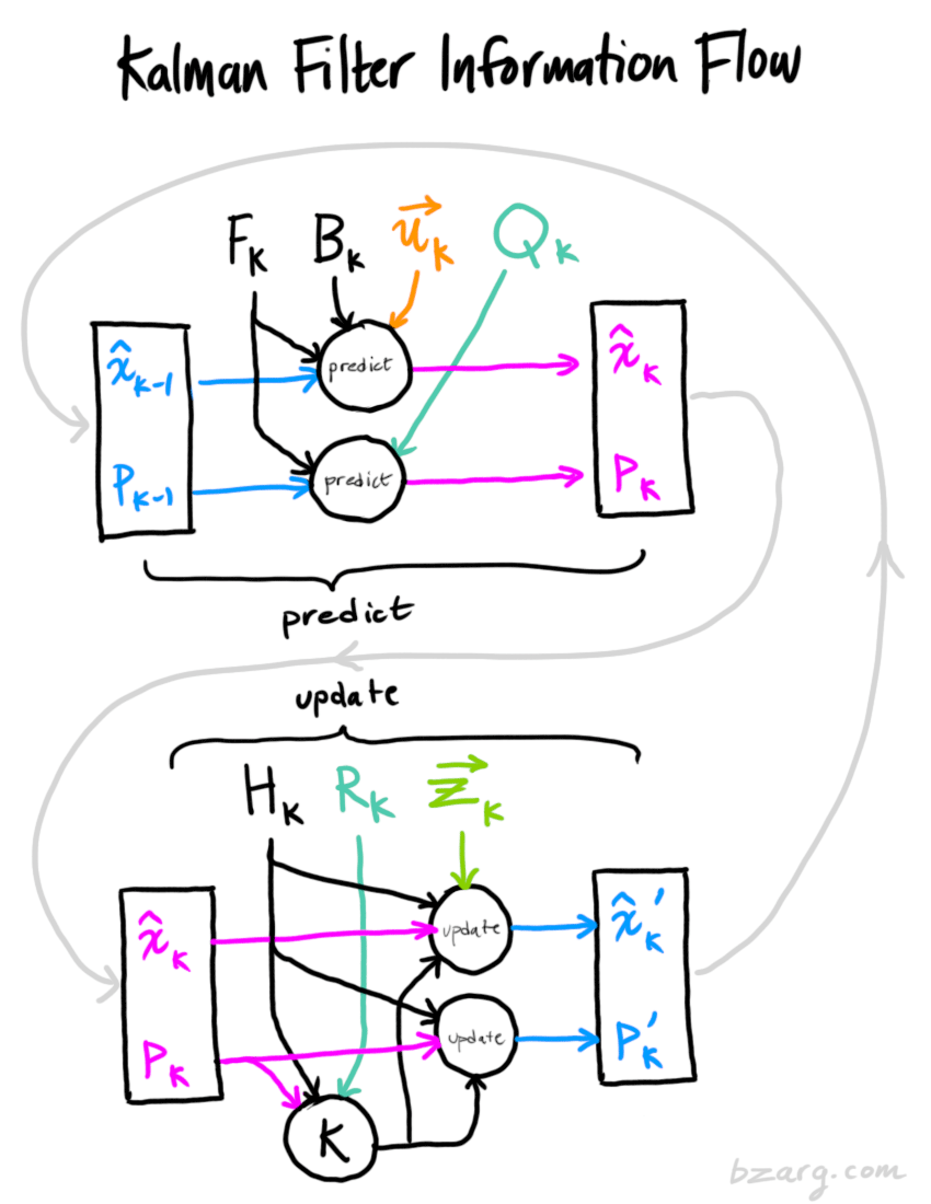
Hey Tim what did you use to draw this illustration?
https://www.bzarg.com/wp-content/uploads/2015/08/kalflow.png
All the illustrations are done primarily with Photoshop and a stylus.
Did you use stylus on screen like iPad or Surface Pro or a drawing tablet like Wacom?
The reason I ask is that latency is still an issue here.
Nice explanation. Looks like someone wrote a Kalman filter implementation in Julia: https://github.com/wkearn/Kalman.jl
Great post! Keep up the good work!
Nice work! I literally just drew half of those covariance diagrams on a whiteboard for someone. Now I can just direct everyone to your page.
Great post. Keep up the good work! I am hoping for the Extended Kalman filter soon.
What happens if your sensors only measure one of the state variables. Do you just make the H matrix to drop the rows you don’t have sensor data for and it all works out?
You reduce the rank of H matrix, omitting row will not make Hx multiplication possible. If in above example only position is measured state u make H = [1 0; 0 0]. If both are measurable then u make H = [1 0; 0 1];
great write up! Thx!!
Very nice, but are you missing squares on those variances in (1)?
Thanks a lot for this wonderfully illuminating article. Like many others who have replied, this too was the first time I got to understand what the Kalman Filter does and how it does it. Thanks a lot
Nice post!
Near ‘You can use a Kalman filter in any place where you have uncertain information’ shouldn’t there be a caveat that the ‘dynamic system’ obeys the markov property? I.e. a process where given the present, the future is independent of the past (not true in financial data for example).
Also just curious, why no references to hidden markov models, the Kalman filter’s discrete (and simpler) cousin?
Don’t know if this question was answered, but, yes, there is a Markovian assumption in the model, as well as an assumption of linearity. But, at least in my technical opinion, that sounds much more restrictive than it actually is in practice. If the system (or “plant”) changes its internal “state” smoothly, the linearization of the Kalman is nothing more than using a local Taylor expansion of that state behavior, and, to some degree, a faster rate of change can be compensated for by increasing sampling rate. As far as the Markovian assumption goes, I think most models which are not Markovian can be transformed into alternate models which are Markovian, using a change in variables and such.
Awesome post! I’m impressed.
Aaaargh!
I wish I’d known about these filters a couple years back – they would have helped me solve an embedded control problem with lots of measurement uncertainty.
Thanks for the great post!
Great article and very informative. Love the use of graphics. I would love to see another on the ‘extended Kalman filter’.
Thanks,
Mike
The same here! And i agree the post is clear to read and understand. Thanks to the author!
Great article, thanks!
It would be great if you could repeat all the definitions just after equations (18) and (19) – I found myself constantly scrolling up & down because I couldn’t remember what z was, etc. etc.
Just before equation (2), the kinematics part, shouldn’t the first equation be about p_k rather than x_k, i.e., position and not the state?
This is an excellent piece of pedagogy. Every step in the exposition seems natural and reasonable. I just chanced upon this post having the vaguest idea about Kalman filters but now I can pretty much derive it. The only thing I have to ask is whether the control matrix/vector must come from the second order terms of the taylor expansion or is that a pedagogical choice you made as an instance of external influence? Also, I guess in general your prediction matrices can come from a one-parameter group of diffeomorphisms.
Nope, using acceleration was just a pedagogical choice since the example was using kinematics. The control matrix need not be a higher order Taylor term; just a way to mix “environment” state into the system state.
I wish there were more posts like this. That explain how amazing and simple ideas are represented by scary symbols. Loved the approach. Can you please do one on Gibbs Sampling/Metropolis Hastings Algorithm as well?
Very nice write up! The use of colors in the equations and drawings is useful.
Small nitpick: an early graph that shows the uncertainties on x should say that sigma is the standard deviation, not the “variance”.
@Eric Lebigot: Ah, yes, the diagram is missing a ‘squared’ on the sigma symbols. I’ll fix that when I next have access to the source file for that image.
Eye opening. The only part I didn’t follow in the derivation, is where the left hand side of (16) came from… until I realized that you defined x’_k and P’_k in the true state space coordinate system, not in the measurement coordinate system – hence the use of H_k!
same question! i dont understand this point too.
Hmm, I didn’t think this through yet, but don’t you need to have a pretty good initial guess for your orientation (in the video example) in order for the future estimates to be accurate? Please show this is not so :)
Great illustration and nice work! Thanks!
(Or is it all “hidden” in the “velocity constrains acceleration” information?)
The Kalman filter is quite good at converging on an accurate state from a poor initial guess. Representing the uncertainty accurately will help attain convergence more quickly– if your initial guess overstates its confidence, the filter may take awhile before it begins to “trust” the sensor readings instead.
In the linked video, the initial orientation is completely random, if I recall correctly. I think it actually converges quite a bit before the first frame even renders. :)
“The math for implementing the Kalman filter appears pretty scary and opaque in most places you find on Google.” Indeed. I’ve tried to puzzle my way through the Wikipedia explanation of Kalman filters on more than one occasion, and always gave up.
I was able to walk through your explanation with no trouble. Thank you.
I’m a PhD student in economics and decided a while back to never ask Wikipedia for anything related to economics, statistics or mathematics because you will only leave feeling inadequate and confused. Seriously, concepts that I know and understand perfectly well look like egyptian hieroglyphs when I look at the wikipedia representation. I would ONLY look at the verbal description and introduction, the formulas seem to all be written by a wizard savant.
The article has a perfect balance between intuition and math! This is the first time I actually understood Kalman filter. =)
I have a couple of questions.
The way we got second equation in (4) wasn’t easy for me to see until I manually computed it from the first equation in (4). Is it meant to be so, or did I missed a simple relation? When you say “I’ll just give you the identity”, what “identity” are you referring to? Are you referring to given equalities in (4)?
So, sensors produce:
– observed noisy mean and covariance (z and R) we want to correct, and
– an additional info ‘control vector’ (u) with known relation to our prediction.
Correct?
Does H in (8) maps physical measurements (e.g. km/h) into raw data readings from sensors (e.g. uint32, as described in some accelerometer’s reference manual)?
(4) was not meant to be derived by the reader; just given.
Z and R are sensor mean and covariance, yes. The control vector ‘u’ is generally not treated as related to the sensors (which are a transformation of the system state, not the environment), and are in some sense considered to be “certain”. For example, the commands issued to the motors in a robot are known exactly (though any uncertainty in the execution of that motion could be folded into the process covariance Q).
Yes, H maps the units of the state to any other scale, be they different physical units or sensor data units. I suppose you could transform the sensor measurements to a standard physical unit before it’s input to the Kalman filter and let H be the some permutation matrix, but you would have to be careful to transform your sensor covariance into that same space as well, and that’s basically what the Kalman filter is already doing for you by including a term for H. (That would also assume that all your sensors make orthogonal measurements, which not necessarily true in practice).
A possible explanation for (4) may be this: https://stats.stackexchange.com/a/498108/322199
However, I still do not have an understanding of what APA^T is doing and how it is different from AP.
So what happens if you don’t have measurements for all DOFs in your state vector? I’m assuming that means that H_k isn’t square, in which case some of the derivation doesn’t hold, right? What do you do in that case?
Excellent explanation. Thanks!
Kalman filters are used in dynamic positioning systems for offshore oil drilling.
Great write up. Very helpful. Thanks.
Just one question. Shouldn’t it be p_k in stead of x_k (and p_k-1 instead of x_k-1) in the equation right before equation (2)? Also, in (2), that’s the transpose of x_k-1, right?
I guess the same thing applies to equation right before (6)?
Regards,
Istvan Hajnal
Yes, my thinking was to make those kinematic equations look “familiar” by using x (and it would be understood where it came from), but perhaps the inconsistency is worse. :\
Great ! Really interesting and comprehensive to read.
Thanks for the post, I have learnt a lot. My background is signal processing, pattern recognition.
One question:
If we have two probabilities and we want to know the chance that both are true, we just multiply them together.
Why not use sum or become Chi-square distribution?
Because from http://math.stackexchange.com/questions/101062/is-the-product-of-two-gaussian-random-variables-also-a-gaussian
The product of two Gaussian random variables is distributed, in general, as a linear combination of two Chi-square random variables.
Thanks,
Regards,
Li
Ah, not quite. Let \(X\) and \(Y\) both be Gaussian distributed. We are not doing \(\text{pdf}(X \cdot Y)\), we are doing \(\text{pdf}(X) \cdot \text{pdf}(Y)\)!
Hello, is there a reason why we multiply the two Gaussian pdfs together? I mean, why not add them up or do convolution or a weighted sum…etc?
And thanks for the great explanations of kalman filter in the post :)
Here is a good explanation whey it is the product of two Gaussian PDF. Basically, it is due to Bayesian principle
https://math.stackexchange.com/q/2630447
Really interesting article. Clear and simple. Exactly what I needed.
Thank you very much for this very clear article!
Great post ! I have a question about fomula (7), How to get Qk genenrally ?
Great post. It demystifies the Kalman filter in simple graphics. A great teaching aid. Thx.
Hello Tim,
Very nice article. I had read the signal processing article that you cite and had given up half way.
This article clears many things. I will now have to implement it myself.
It would be nice if you could write another article with an example or maybe provide Matlab or Python code.
Keep up the good work.
Best Regards
Chintan
Awesome post!!! Great visuals and explanations.
Can you realy knock an Hk off the front of every term in (16) and (17) ?
I think this operation is forbidden for this matrix.
Wow! This post is amazing. It really helps me to understand true meaning behind equations.
This is simplyy awesum!!!! this demonstration has given our team a confidence to cope up with the assigned project
Great post! Thanks
Amazing article, I struggled over the textbook explanations. This article summed up 4 months of graduate lectures, and i finally know whats going on. Thank you.
Greta article, thank you!
Great work. Thanks!
Hello,
This is indeed a great article. I have been trying to understand this filter for some time now. This article makes most of the steps involved in developing the filter clear.
I how ever did not understand equation 8 where you model the sensor. What does the parameter H do here. How do you obtain the components of H.
Thanks in advance,
Jose
Very good job explaining and illustrating these! Now I understand how the Kalman gain equation is derived. It was hidden inside the properties of Gaussian probability distributions all along!
This is the greatest explanation ever!
Great explanation! I have a question though just to clarify my understanding of Kalman Filtering. In the above example (position, velocity), we are providing a constant acceleration value ‘a’. Assuming this is a car example, let’s say the driver decides to change the acceleration during the trip. From what I understand of the filter, I would have to provide this value to my Kalman filter for it to calculated the predicted state every time I change the acceleration. Kalman filter would be able to “predict” the state without the information that the acceleration was changed. Is this correct? Also, would this be impractical in a real world situation, where I may not always be aware how much the control (input) changed?
Can anyone help me with this?
you are the best Tim!
thank you very much
hey, my kalman filter output is lagging the original signal. However it does a great job smoothing. How does lagging happen
I must say the best link in the first page of google to understand Kalman filters. I guess I read around 5 documents and this is by far the best one. Well done and thanks!! cheers!! :D
Excellent explanation.
After reading many times about Kalman filter and giving up on numerous occasions because of the complex probability mathematics, this article certainly keeps you interested till the end when you realize that you just understood the entire concept.
Keep up the good work.
Thank you for your excelent work!
There is no doubt, this is the best tutorial about KF !
Many thanks!
Great article ! Clear and easy to understand.
This is by far the best explanation of a Kalman filter I have seen yet. Very well done.
v.nice explanation. Actually I have something different problem if you can provide a solution to me. In my system, I have starting and end position of a robot. I need to find angle if robot needs to rotate and velocity of a robot. Can I get solution that what will be Transition matrix, x(k-1), b(k), u(k).
Thanks Baljit
Such an amazing explanation of the much scary kalman filter. Kudos to the author. Thanks very much Sir. Expecting such explanation for EKF, UKF and Particle filter as well.
Hello There!
Great article but I have a question. Why did you consider acceleration as external influance? Could we add the acceleration inside the F matrix directly e.g. x=[position, velocity, acceleration]’ ?
Thanks!
I think that acceleration was considered an external influence because in real life applications acceleration is what the controller has (for lack of a better word) control of. In other words, acceleration and acceleration commands are how a controller influences a dynamic system.
Thank you so so much Tim. The math in most articles on Kalman Filtering looks pretty scary and obscure, but you make it so intuitive and accessible (and fun also, in my opinion). Again excellent job! Would you mind if I share part of the particles to my peers in the lab and maybe my students in problem sessions? I’ll certainly mention the source
Best explanation I’ve read so far on the Kalman filter. Far better than many textbooks. Thank you.
Without doubt the best explanation of the Kalman filter I have come across! Often in DSP, learning materials begin with the mathematics and don’t give you the intuitive understanding of the problem you need to fully grasp the problem. This is a great resource. Thanks.
amazing…simply simplified.you saved me a lot of time…thanks for the post.please update with nonlinear filters if possible that would be a great help.
Your original approach (is it ?) of combining Gaussian distributions to derive the Kalman filter gain is elegant and intuitive. All presentations of the Kalman filter that I have read use matrix algebra to derive the gain that minimizes the updated covariance matrix to come to the same result. That was satisfying enough to me up to a point but I felt i had to transform X and P to the measurement domain (using H) to be able to convince myself that the gain was just the barycenter between the a priori prediction distribution and the measurement distributions weighted by their covariances. This is where other articles confuse the reader by introducing Y and S which are the difference z-H*x called innovation and its covariance matrix. Then they have to call S a “residual” of covariance which blurs understanding of what the gain actually represents when expressed from P and S. Good job on that part !
I will be less pleasant for the rest of my comment, your article is misleading in the benefit versus effort required in developing an augmented model to implement the Kalman filter. By the time you invested the research and developing integrated models equations for errors of your sensors which is what the KF filter is about, not the the recursive algorithm principle presented here which is trivial by comparison.
There is nothing magic about the Kalman filter, if you expect it to give you miraculous results out of the box you are in for a big disappointment. By the time you have developed the level of understanding of your system errors propagation the Kalman filter is only 1% of the real work associated to get those models into motion. There is a continuous supply of serious failed Kalman Filters papers where greedy people expect to get something from nothing implement a EKF or UKF and the result are junk or poor. All because of article like yours give the false impression that understanding a couple of stochastic process principles and matrix algebra will give miraculous results. The work in not where you insinuate it is. Understanding the Kalman filter predict and update matrix equation is only opening a door but most people reading your article will think it’s the main part when it is only a small chapter out of 16 chapters that you need to master and 2 to 5% of the work required.
Great article I’ve ever been reading on subject of Kalman filtering. Thanks !!!
fantastic | thanks for the outstanding post !
First time am getting this stuff…..it doesn’t sound Greek and Chinese…..greekochinese…..
on point….and very good work…..
thank you Tim for your informative post, I did enjoy when I was reading it, very easy and logic… good job
Equation 18 (measurement variable) is wrong.
Equation 16 is right. Divide all by H.
What’s the issue? Note that K has a leading H_k inside of it, which is knocked off to make K’.
x has the units of the state variables.
z has the units of the measurement variables.
K is unitless 0-1.
The units don’t work unless the right term is K(z/H-x).
Excellent Post! Kalman Filter has found applications in so diverse fields. A great one to mention is as a online learning algorithm for Artificial Neural Networks.
Great Article. Nicely articulated. Do you recommened any C++ or python implementation of kalman filter? I know there are many in google but your recommendation is not the same which i choose.
Assume that every car is connected to internet. I am trying to predict the movement of bunch of cars, where they probably going in next ,say 15 min. you can assume like 4 regions A,B,C,D (5-10km of radius) which are close to each other. How can I make use of kalman filter to predict and say, so many number cars have moved from A to B.
I am actullay having trouble with making the Covariance Matrix and Prediction Matrix. In my case I know only position. Veloctiy of the car is not reported to the cloud. So First step could be guessing the velocity from 2 consecutive position points, then forming velocity vector and position vector.Then applying your equations. Is my assumption is right? Thanks
P.S: sorry for the long comment.Need Help. Thanks
Excellent Post! thanks alot.
I want to use kalman Filter to auto correct 2m temperature NWP forecasts.
Could you please help me to get a solution or code in R, FORTRAN or Linux Shell Scripts(bash,perl,csh,…) to do this.
Hi
I’m kinda new to this field and this document helped me a lot
I just have one question and that is what is the value of the covariance matrix at the start of the process?
This is the best article I’ve read on Kalman filter so far by a long mile!
Btw, will there be an article on Extend Kalman Filter sometime in the future, soon hopefully?
Thanks! Great work
Thanks a bunch. :) Very helpful indeed
Thanks a lot :D Great article!
Awesome thanks! :)
My main interest in the filter is its significance to Dualities which you have not mentioned – pity
Thank you for the really good work!
Excellent. Thank you.
Excellent explanation! best I can find online for newbies! Pls do a similar one for UKF pls!
This article completely fills every hole I had in my understanding of the kalman filter. Thank you so much!
Pure Gold !
Thanks!
Great work. The explanation is really very neat and clear.
RIP Rudolf E. Kálmán.
Awsm work. kalman filter was not that easy before. Thanks a lot.
Great article. I used this filter a few years ago in my embedded system, using code segments from net, but now I finally understand what I programmed before blindly :). Thanks.
PURE AWESOMENESS!
Thanks.
Amazing! Funny and clear! Thanks a lot! It definitely give me a lot of help!!!!
very helpful thanks
This is great actually. Im studying electrial engineering (master). Ive read plenty of Kalman Filter explanations and derivations but they all kinda skip steps or forget to introduce variables, which is lethal.
I had to laugh when I saw the diagram though, after seeing so many straight academic/technical flow charts of this, this was refreshing :D
If anyone really wants to get into it, implement the formulas in octave or matlab then you will see how easy it is. This filter is extremely helpful, “simple” and has countless applications.
Awesome! Acquisition of techniques like this might end up really useful for my robot builder aspirations… *sigh* *waiting for parts to arrive*
An excellent way of teaching in a simplest way.
Thank you so much, that was really helpful . AMAZING
Excellent tutorial on kalman filter, I have been trying to teach myself kalman filter for a long time with no success. But I actually understand it now after reading this, thanks a lot!!
Thank you very much for your explanation. This is the best tutorial that I found online. I’m also expect to see the EKF tutorial. Thank you!!!
Hi, dude,
great article.
there is a typo in eq(13) which should be \sigam_1 instead of \sigma_0.
Nope, that would give the wrong answer. See the same math in the citation at the bottom of the article.
Please write your explanation on the EKF topic as soon as possible…, or please tell me the recommended article about EKF that’s already existed by sending the article through the email :) (or the link)
Thank you for this excellent post. Just one detail: the fact that Gaussians are “simply” multiplied is a very subtle point and not as trivial as it is presented, see http://stats.stackexchange.com/questions/230596/why-do-the-probability-distributions-multiply-here.
Great question! It has confused me a long time
Just another big fan of the article. Great job! I definitely understand it better than I did before.
Oh my god. Thank you so much for this. Until now, I was totally and completely confused by Kalman filters. The pictures and examples are SO helpful. THANK YOU!!!
Thank you so much for this explaination.
Love it – thank you M. Bzarg! I owe you a significant debt of gratitude…
Many thanks for this article,
sometimes the easiest way to explain something is really the harthest!
You did it!
Good job,thank you so much!
This is a great explanation. The one thing that you present as trivial, but I am not sure what the inuition is, is this statement:
“””
This is where we need another formula. If we multiply every point in a distribution by a matrix A, then what happens to its covariance matrix Σ?
Well, it’s easy. I’ll just give you the identity:
Cov(x)=Σ
Cov(Ax)==AΣA^T
“””
Why is that easy? Thanks so much for your effort!
It’s easy because I gave it to you. :)
I think of it in shorthand – and I could be wrong – as
— you spread state x out by multiplying by A
— sigma is the covariance of the vector x (1d), which spreads x out by multiplying x by itself into 2d
so
— you spread the covariance of x out by multiplying by A in each dimension ; in the first dimension by A, and in the other dimension by A_t
Thanks for making science and math available to everyone!
On mean reverting linear systems how can I use the Kalman filter to measure the half life of mean reversion?
Hey!
Just wanted to give some feedback. I really enjoyed your explanation of Kalman filters. Also, thank you very much for the reference!
Thanks for a good tutorial !! What does a accelerometer cost to the Arduino? :D
I have never come across so beautifully and clearly elaborated explanation for Kalman Filter such as your article!! Thanks a lot for giving a lucid idea about Kalman Filter! Do continue to post many more useful mathematical principles
Hey!
Thanks for the great article. I have a couple of questions though:
1) Why do we multiply the state vector (x) by H to make it compatible with the measurements. Why don’t we do it the other way around? Would there be any issues if we did it the other way around?
2) If you only have a position sensor (say a GPS), would it be possible to work with a PV model as the one you have used? I understand that we can calculate the velocity between two successive measurements as (x2 – x1/dt). I just don’t understand where this calculation would be fit in.
Thanks :)
I am currently working on my undergraduate project where I am using a Kalman Filter to use the GPS and IMU data to improve the location and movements of an autonomous vehicle. I would like to know what was in Matrix A that you multiplied out in equations 4 and 5. Thank you for the helpful article!
The matrix A is just an example in equation 4, it is F_k in the equation 5. ( A = F_k )
Great article Thank you!
Thanks for making math accessible to us. I wish more math topics were presented this well.
Very cool article! Thank you!
Awesome post. Thanks a lot !
Thank you for your amazing work!
but i have a question please !
why this ??
We can knock an Hk off the front of every term in (16) and (17) (note that one is hiding inside K ), and an HTk off the end of all terms in the equation for P′k.
very nice! thanks!
excellent job, thanks a lot for this article.
I know I am very late to this post, and I am aware that this comment could very well go unseen by any other human eyes, but I also figure that there is no hurt in asking. This article was very helpful to me in my research of kalman filters and understanding how they work. I would absolutely love if you were to do a similar article about the Extended Kalman filter and the Unscented Kalman Filter (or Sigma Point filter, as it is sometimes called). If you never see this, or never write a follow up, I still leave my thank you here, for this is quite a fantastic article.
I cannot express how thankful am I to you. I have an interview and i was having trouble in understanding the Kalman Filter due to the mathematical equations given everywhere but how beautifully have you explained Sir!! I understood each and every part and now feeling so confident about the Interview. Thanks to you
Thank you very much..This article is really amazing
I have been working on Kalman Filter , Particle Filter and Ensemble Kalman Filter for my whole PhD thesis, and this article is absolutely the best tutorial for KF I’ve ever seen. I’m looking forward to read your article on EnKF.
One thing may cause confusion this the normal * normal part. The product of two independent normals are not normal. It should be better to explained as: p(x | z) = p(z | x) * p(x) / p(z) = N(z| x) * N(x) / normalizing constant.
Awesome. I felt something was at odds there too. anderstood in the previous reply also shared the same confusion. I was about to reconcile it on my own, but you explained it right! Thanks!
Thanks a lot for the nice and detailed explanation!
After years of struggling to catch the physical meaning of all those matrices, evereything is crystal clear finally!
THANK YOU MAN, I LOVE YOU
Nice article!
it seems a C++ implementation of a Kalman filter is made here :
https://github.com/hmartiro/kalman-cpp
what amazing description………thank you very very very much
Very good and clear explanation ! Many kudos !
For me the revelation on what kalman is came when I went through the maths for a single dimensional state (a 1×1 state matrix, which strips away all the matrix maths). When you do that it’s pretty clear it’s just the weighed average between the model and the sensor(s), weighted by their error variance.
It also explains how kalman filters can have less lag. You can’t have a filter without lag unless you can predict the future, since filters work by taking into account multiple past inputs. However, with kalman the model is a a kind of “future” prediction (provided your model is good enough).
Thank you for this article. It is very nice and helpful. One of the best teaching tips I picked up from this is coloring equations to match the colored description. Brilliant!
When you knock off the Hk matrix, that makes sense when Hk has an inverse. Is the result the same when Hk has no inverse? In this case, how does the derivation change?
Excellent ! You explained it clearly and simple. Thanks a lot!
Awesome work !! . can you explain particle filter also?
You explained it clearly and simplely. I had not seen it. Tks very much!
It’s great post. But I have one question.
In equation (16), Where did the left part come from? Updated state is already multiplied by measurement matrix and knocked off? I couldn’t understand this step.
Thanks a lot! This is probably the best explanation of KF anywhere in the literature/internet.
Really fantastic explanation of something that baffles a lot of people (me included). Well done!
So damn good! This is the first time that I finally understand what Kalman filter is doing.
I am a University software engineering professor, and this explanation is one of the best I have seen, thanks for your outstanding work.
Where have you been all my life!!!! Finally got it!!!
This is al kinds of awesome.
Great write-up! Thanks!
Loving the explanation.
A great refresher…
This is an amazing explanation; took me an hour to understand what I had been trying to figure out for a week.
One question:
what exactly does H do? Can you give me an example of H? I was assuming that the observation x IS the mean of where the real x could be, and it would have a certain variance. But instead, the mean is Hx. Why is that? why is the mean not just x?
Thanks!
Thanks for the KF article. Very interesting!
Impressive and clear explanation of such a tough subject! Really loved the graphical way you used, which appeals to many of us in a much more significant way. Bravo!
Great work! Thank you so much!
But I have a simple problem. In pratice, we never know the ground truth, so we should assign an initial value for Pk. And my problem is Pk and kalman gain k are only determined by A,B,H,Q,R, these parameters are constant. Therefore, as long as we are using the same sensor(the same R), and we are measuring the same process(A,B,H,Q are the same), then everybody could use the same Pk, and k before collecting the data. Am I right?
Veeeery nice article! One of the best, if not the best, I’ve found about kalman filtering! Makes it much easier to understand! Thanks a lot for your great work!
Thank you for this clear explanation!!
This is an amazing introduction! I read it through and want to and need to read it against. But cannot suppress the inner urge to thumb up!
Hello!
I have acceleration measurements only.How do I estimate position and velocity?
What will be my measurement matrix?
Is it possible to construct such a filter?
Your tutorial of KF is truely amazing. Every material related to KF now lead and redirect to this article (orginal popular one was Kalman Filter for dummies). Hope to see your EKF tutorial soon. Thank you.
Amazing post! Thank you! I guess you did not write the EKF tutorial, eventually?
Small question, if I may:
What if the sensors don’t update at the same rate? You want to update your state at the speed of the fastest sensor, right? Do you “simply” reduce the rank of the H matrix for the sensors that haven’t been updated since the last prediction?
Hey, nice article. I enjoyed reading it. One small correction though: the figure which shows multiplication of two Gaussians should have the posterior be more “peaky” i.e. less variance than both the likelihood and the prior. The blue curve should be more certain than the other two.
Very well explained!! Thank you.
Could you pleaseeeee extend this to the Extended, Unscented and Square Root Kalman Filters as well.
I’m currently studying mechatronics and robotics in my university and we just faced the Kalman Filter. It was really difficult for me to give a practical meaning to it, but after I read your article, now everything is clear!
Really a great one, I loved it!
perfect work, simple and elegant!
Thanks Tim, nice explanation on KF ..really very helpful..looking forward for EKF & UKF
Best Guide on KF ever !
That was fascinating
Thanks
For the extended Kalman Filter:
‘The Extended Kalman Filter: An Interactive Tutorial for Non-Experts’
https://home.wlu.edu/~levys/kalman_tutorial/
(written to be understood by high-schoolers)
I had read an article about simultaneously using 2 same sensors in kalman filter, do you think it will work well if I just wanna measure only the direction using E-compass?? What are those inputs then and the matrix H?
Thanks, great article!
This is great. Such a wonderful description. Can you point me towards somewhere that shows the steps behind finding the expected value and SD of P(x)P(y), with normalisation. I’m getting stuck somewhere
I don’t have a link on hand, but as mentioned above some have gotten confused by the distinction of taking pdf(X*Y) and pdf(X) * pdf(Y), with X and Y two independent random variables. It is the latter in this context, as we are asking for the probability that X=x and Y=y, not the probability of some third random variable taking on the value x*y.
Really clear article. Wish there were more explanations like this one.
great job! best explanation so far
Absolutely brilliant exposition!!! Thank you for the fantastic job of presenting the KF in such a simple and intuitive way.
I could be totally wrong, but for the figure under the section ‘Combining Gaussians’, shouldn’t the blue curve be taller than the other two curves? The location of the resulting ‘mean’ will be between the earlier two ‘means’ but the variance would be lesser than the earlier two variances causing the curve to get leaner and taller.
Yes, the variance is smaller. The blue curve is drawn unnormalized to show that it is the intersection of two statistical sets. I’ve added a note to clarify that, as I’ve had a few questions about it. Thanks for your comment!
That totally makes sense. Thanks for clarifying that bit.
And did I mention you are brilliant!!!? :-)
Great article, I read several other articles on Kalman filter but could not understand it clearly.
However, one question still remains unanswered is how to estimate covariance matrix. It would be great if you could share some simple practical methods for estimation of covariance matrix.
Very Nice Explanation..
Thanks for your effort
thank you … it is a very helpful article
hope the best for you ^_^
Very nice explanation and overall good job ! Thanks !
Nice explanation. I understood everything expect I didn’t get why you introduced matrix ‘H’. Can you please explain it?
Thanks,
Krishna
Perhaps, the sensor reading dimensions (possibly both scale and units) are not consistent with what you are keeping track of and predict……….as the author had previously alluded to that these sensor readings are might only ‘indirectly’ measure these variables of interest. Say, the sensors are measuring acceleration and then you are leveraging these acceleration measurements to compute the velocity (you are keeping track of) ; and same holds true with the other sensor. Since, there is a possibility of non-linear relationship between the corresponding parameters it warrants a different co-variance matrix and the result is you see a totally different distribution with both mean and co-variance different from the original distribution. So, essentially, you are transforming one distribution to another consistent with your setting.
Hope this makes sense.
H puts sensor readings and the state vector into the same coordinate system, so that they can be sensibly compared.
In the simplest case, H can be biases and gains that map the units of the state vector to the units of the sensors. In a more complex case, some element of the state vector might affect multiple sensor readings, or some sensor reading might be influenced by multiple state vector elements. For example, a craft’s body axes will likely not be aligned with inertial coordinates, so each coordinate of a craft’s interial-space acceleration vector could affect all three axes of a body-aligned accelerometer.
Bonjour,
i need to implémet a banc of 4 observers (kalman filter) with DOS( Dedicated observer), in order to detect and isolate sensors faults
each observer is designed to estimate the 4 system outputs qu’une seule sortie par laquelle il est piloté, les 3 autres sorties restantes ne sont pas bien estimées, alors que par définition de la structure DOS, chaque observateur piloté par une seule sortie et toutes les entrées du système doit estimer les 4 sorties.
SVP veuillez m’indiquer comment faire pour résoudre ce problème et merci d’avance
How I can get Q and R? Can somebody show me exemple.
I can’t figure this out either. Are Q and R vectors? Matrices? Great article! I can almost implement one, but I just cant figure out R & Q.
Q and R are covariances of noise, so they are matrices. Their values will depend on the process and uncertainty that you are modeling.
In many cases the best you can do is measure them, by performing a repeatable process many times, and recording a population of states and sensor readings. You can then compute the covariance of those datasets using the standard algorithm.
I’d like a cookbook demonstration.
ie say: simple sensor with arduino and reduced testcase or absolute minimal C code
tx ~:”
Excellent article on Kalman Filter.
Thank you very much.
But I still have a question, why use multiply to combine Gaussians?
Maybe it is too simple to verify.
Really COOL. I understand Kalman Filter now. Thanks very much!
Amazing article! Explained very well in simple words!
Thanks so much!
I wanted to clarify something about equations 3 and 4. You give the following equation to find the next state;
Xk=FkXk-1 (equation 3)
You then use the co-variance identity to get equation 4.
Cov(AX) = AEA^t
For Cov(X)= E, are you saying that Cov(X-1) = Pk-1?
Is this the reason why you get Pk=Fk*Pk-1*Fk^T? because Fk*Xk-1 is just Xk therefore you get Pk rather than Pk-1? in equation 5 as F is the prediction matrix?
F is the prediction matrix, and \(P_{k-1}\) is the covariance of \(x_{k-1}\).
I have not finish to read the whole post yet, but I couldn’t resist saying I’m enjoying by first time reading an explanation about the Kalman filter. I felt I need to express you my most sincere congratulations. I’ll add more comments about the post when I finish reading this interesting piece of art.
Pd. I’m sorry for my pretty horrible English :(
Ok. I have read the full article and, finally, I have understood this filter perfectly and I have applied it to my researches successfully. Thank you so much Tim!
Super excellent demultiplexing of the Kalman Filter through color coding and diagrams!
Thank you very much for this lovely explanation.
Can you please explain:
1. How do we initialize the estimator ?
2. How does the assumption of noise correlation affects the equations ?
3. How can we see this system is linear (a simple explanation with an example like you did above would be great!) ?
Fantastic article, really enjoyed the way you went through the process.
One question, will the Kalman filter get more accurate as more variables are input into it? ie. if you have 1 unknown variable and 3 known variables can you use the filter with all 3 known variables to give a better prediction of the unknown variable and can you keep increasing the known inputs as long as you have accurate measurements of the data.
Mostly thinking of applying this to IMUs, where I know they already use magnetometer readings in the Kalman filter to remove error/drift, but could you also use temperature/gyroscope/other readings as well? Or do IMUs already do the this?
You are awesome
Thanks for this article, it was very useful. Here’s an observation / question:
The prediction matrix F is obviously dependent on the time step (delta t). It also appears the external noise Q should depend on the time step in some way. e.g. if Q is constant, but you take more steps by reducing delta t, the P matrix accumulates noise more quickly. It appears Q should be made smaller to compensate for the smaller time step.
Do you know of a way to make Q something like the amount of noise per second, rather than per step?
Very well explained. I found many links about Kalman which contains terrifying equations and I ended up closing every one of them. This article really explains well the basic of Kalman filter.
Great article!! Even though I already used Kalman filter, I just used it. By this article, I can finally get knowledges of Kalman filter.
Hi, Great article and great images !
you should mention how to initialize the covariance matrices.
I implemented my own and I initialized Pk as P0=[1 0; 0 1]. Pk will then converge by itself.
I initialized Qk as Q0=[0 0; 0 varA], where varA is the variance of the accelerometer. varA is estimated form the accelerometer measurement of the noise at rest.
Same for Rk, I set it as Rk=varSensor. The estimated variance of the sensor at rest.
ps. to get the variance of few measure points at rest, let’s call them xi={x1, x2, … xn}
first get the mean as: mean(x)=sum(xi)/n
then the variance is given as: var(x)=sum((xi-mean(x))^2)/n
see here (scroll down for discrete equally likely values): https://en.wikipedia.org/wiki/Variance
Cheers,
Romain
THANK YOU KIND SIR! :)
This is definitely one of the best explanations of KF I have seen! I am trying to explain KF/EKF in my master thesis and I was wondering if I could use some of the images! They’re really awesome!
Cheers,
Aditya
Hello! Equation 12 results in a scalar value….just one value as the result. But equation 14 involves covariance matrices, and equation 14 also has a ‘reciprocal’ symbol. Could you please explain whether equation 14 is feasible (correct)? That is, if we have covariance matrices, then it it even feasible to have a reciprocal term such as (sigma0 + sigma1)^-1 ?
Hello. I’d like to add…… when I meant reciprocal term in equation 14, I’m talking about (sigma0 + sigma1)^-1…. which appears to be 1/[sigma0 + sigma1]. But if sigma0 and sigma1 are matrices, then does that fractional reciprocal expression even make sense? Just interested to find out how that expression actually works, or how it is meant to be interpreted – in equation 14. Thanks.
Simply, Great Work!!
Thank you so much :)
Nice article, it is the first time I go this far with kalman filtering (^_^;)
Would you mind to detail the content (and shape) of the Hk matrix, if the predict step have very detailed examples, with real Bk and Fk matrices, I’m a bit lost on the update step.
What is Hk exactly, what if my mobile have two sensors for speed for example and one very noisy for position…
Wow..
FINALLY found THE article that clear things up!
Thanks for the awesome article!
Very well explained, one of the best tutorials about KF so far, very easy to follow, you’ve perfectly clarified everything, thank you so much :)
Finally found out the answer to my question, where I asked about how equations (12) and (13) convert to a matrix form of equation (14). The answer is …… it’s not a simple matter of taking (12) and (13) to get (14). The theory for obtaining a “kalman gain MATRIX” K is much more involved than just saying that (14) is the ‘matrix form’ of (12) and (13). So, if anybody here is confused about how (12) and (13) converts to (14) and (14), I don’t blame you, because the theory for that is not covered here.
This particular article, however….. is one of the best I’ve seen though. It is one that attempts to explain most of the theory in a way that people can understand and relate to.
Finally found out the answer to my question, where I asked about how equations (12) and (13) convert to a matrix form of equation (14). The answer is …… it’s not a simple matter of taking (12) and (13) to get (14). The theory for obtaining a “kalman gain MATRIX” K is much more involved than just saying that (14) is the ‘matrix form’ of (12) and (13). So, if anybody here is confused about how (12) and (13) converts to (14) and (15), I don’t blame you, because the theory for that is not covered here.
This particular article, however….. is one of the best I’ve seen though. It is one that attempts to explain most of the theory in a way that people can understand and relate to.
Thank you. :) Love your illustrations and explanations. Made things much more clear. Please draw more robots. XD
I only understand basic math and a lot of this went way over my head. I’m making a simple two wheel drive microcontroller based robot and it will have one of those dirt cheap 6-axis gyro/accelerometers. Was looking for a way to extract some sense and a way to combine this sensor data into meaningful data that can be used to steer the robot. There’re a lot of uncertainties and noise in such system and I knew someone somewhere had cracked the nut. Now I know at least some theory behind it and I’ll feel more confident using existing programming libraries that Implement these principles.
Even though I don’t understand all in this beautiful detailed explanation, I can see that it’s one of the most comprehensive. I appreciate your time and huge effort put into the subject. Bookmarked and looking forward to return to reread as many times as it takes to understand it piece by piece.
Great blog!! Thanks to your nice work!
By the way, can I translate this blog into Chinese? Of course, I will put this original URL in my translated post. :)
Thank you! this clarified my question abou the state transition matrix. Most people may be satisfied with this explanation but I am not.
I am still curious about examples of control matrices and control vectors – the explanation of which you were kind enough to gloss over in this introductory exposition.
I have a lot of other questions and any help would be appreciated!
I have a strong background in stats and engineering math and I have implemented K Filters and Ext K Filters and others as calculators and algorithms without a deep understanding of how they work. I would like to get a better understanding please with any help you can provide. Thank you!
what if we don’t have the initial velocity.
yes i can use the coordinates ( from sensor/LiDAR ) of first two frame to find the velocity but that is again NOT completely reliable source
what should i do???
I did not understand what exactly is H matrix. Can you explain the difference between H,R,Z?
i am doing my final year project on designing this estimator, and for starters, this is a good note and report ideal for seminar and self evaluating,. thanks admin for posting this gold knowledge. made easy for testing and understanding in a simple analogy. with great graphs and picture content. couldnt thank less. peace.
This is so helpful!!!
A big question here is …. in equation (6), why is the projection (ie. xk) calculated from the state matrix Fk (instead of F_k-1 ? Similarly? Why Bk and uk?
If we’re trying to get xk, then shouldn’t xk be computed with F_k-1, B_k-1 and u_k-1? It is because, when we’re beginning at an initial time of k-1, and if we have x_k-1, then we should be using information available to use for projecting ahead…. which means F_k-1, B_k-1 and u_k-1, right? Not F_k, B_k and u_k.
\(F_{k}\) is defined to be the matrix that transitions the state from \(x_{k-1}\) to \(x_{k}\). We could label it \(F_{k-1}\) and it would make no difference, so long as it carried the same meaning.
Similarly \(B_k\) is the matrix that adjusts the final system state at time \(k\) based on the control inputs that happened over the time interval between \(k-1\) and \(k\). We could label it however we please; the important point is that our new state vector contains the correctly-predicted state for time \(k\).
We also don’t make any requirements about the “order” of the approximation; we could assume constant forces or linear forces, or something more advanced. The only requirement is that the adjustment be represented as a matrix function of the control vector.
Hi tbabb! Thanks for your kind reply. And thanks very much for explaining. I was only coming from the discrete time state space pattern:
x[k+1] = Ax[k] + Bu[k]. I assumed that A is Ak, and B is Bk.
Then, when re-arranging the above, we get:
x[k] = Ax[k-1] + Bu[k-1]. I assumed here that A is A_k-1 and B is B_k-1. This suggests order is important. But, on the other hand, as long as everything is defined …. then that’s ok. Thanks again! Nice site, and nice work.
The article was really great. It helped me understand KF much better. But I still have a doubt about how you visualize senor reading after eq 8. There are two visualizations, one in pink color and next one in green color. Can you explain the relation/difference between the two ?
Thanks in advance.
Needless to say, concept has been articulated well and serves it purpose really well!
I could get how matrix Rk got introduced suudenly
(μ1,Σ1)=(zk→,Rk) .
I think I need read it again,
Explanation of Kalman Gain is superb.
Thanks a lot
The explanation is great but I would like to point out one source of confusion which threw me off. P_k should be the co-variance of the actual state and the truth and not co-variance of the actual state x_k. This will make more sense when you try deriving (5) with a forcing function.
Superb ! Very simply and nicely put. Thanks a lot !!
This is, by far, the best tutorial on Kalman filters I’ve found. You provided the perfect balance between intuition and rigorous math. Thank you :)
Hello, thank you for this great article. I followed it and would like to code something up but I am stopped at the computation of the Covariance matrix. I understand that each summation is integration of one of these: (x*x)* Gaussian, (x*v)*Gaussian, or (v*v)*Gaussian . I can use integration by parts to get down to integration of the Gaussian but then I run into the fact that it seems to be an integral that wants to result in the Error function, but the bounds don’t match. It only works if bounds are 0 to inf, not –inf to inf. So I am unable to integrate to form the Covariance matrix. Could you please point me in the right direction. Thanks!
Now i understood, you are great!
Great Job!!! Really the best explonation of Kalman Filter ever! Now my world is clear xD Is really not so scary as it’s shown on Wiki or other sources! Thank You very much!
hi, i would like to ask if it possible to add the uncertainty in term of magnetometer, gyroscope and accelerometer into the kalman filter?
Wow, fantastic article.
Very neat! Thanks for this article.
Excellent article and very clear explanations. I love your graphics. Thank you very much.
I really would like to read a follow-up about Unscented KF or Extended KF from you.
Thanks for this article. Super! Simple and clear!
Thanks for your article, you ‘ve done a great job mixing the intuitive explanation with the mathematical formality. Now I can finally understand what each element in the equation represents.
In “Combining Gaussians” section, why is the multiplication of two normal distributions also a normal distribution. This doesn’t seems right if the two normal distributions are not independent.
really great post: easy to understand but mathematically precise and correct. Thank you!
Very great explaination and really very intuitive. excited to see your other posts from now on.
Informative Article.. It will be great if you provide the exact size it occupies on RAM,efficiency in percentage, execution of algorithm
so great article, I have question about equation (11) and (12). could you explain it or another source that i can read?
Fantastic! Thanks for your explanation!
” (being careful to renormalize, so that the total probability is 1) ”
Can someone be kind enough to explain that part to me ? How do you normalize a Gaussian distribution ? Sorry for the newby question, trying to undertand the math a bit.
Thanks in advance
The integral of a distribution over it’s domain has to be 1 by definition. Also, I don’t know if that comment in the blog is really necessary because if you have the covariance matrix of a multivariate normal, the normalizing constant is known: det(2*pi*(Covariance Matrix))^(-1/2). There’s nothing to really be careful about. See https://en.wikipedia.org/wiki/Multivariate_normal_distribution
Amazing article! Very impressed! You must have spent some time on it, thank you for this!
I had one quick question about Matrix H. Can it be extended to have more sensors and states? For example say we had 3 sensors, and the same 2 states, would the H matrix look like this:
H = [ [Sensor1-to-State 1(vel) conversion Eq , Sensor1-to-State 2(pos) conversion Eq ] ;
[Sensor2-to-State 1(vel) conversion Eq , Sensor2-to-State 2(pos) conversion Eq ] ;
[Sensor3-to-State 1(vel) conversion Eq , Sensor3-to-State 2(pos) conversion Eq ] ]
Thank you!
Simply love it.
Hey Author,
Good work. Can you elaborate how equation 4 and equation 3 are combined to give updated covariance matrix?
\(F_k\) is a matrix applied to a random vector \(x_{k-1}\) with covariance \(P_{k-1}\). Equation (4) says what we do to the covariance of a random vector when we multiply it by a matrix.
Simply Awesome!
This article is the best one about Kalman filter ever. Thanks for your help.
But I have a question about how to do knock off Hk in equation (16), (17).
Because usual case Hk is not invertible matrix, so i think knocking off Hk is not possible.
Can you explain?
Mind Blown !! The fact that you perfectly described the reationship between math and real world is really good. Thnaks a lot!!
Can this method be used accurately to predict the future position if the movement is random like Brownian motion.
If you have sensors or measurements providing some current information about the position of your system, then sure.
In the case of Brownian motion, your prediction step would leave the position estimate alone, and simply widen the covariance estimate with time by adding a constant \(Q_k\) representing the rate of diffusion. Your measurement update step would then tell you to where the system had advanced.
It is an amazing article, thank you so much for that!!!!!
Is the method useful for biological samples variations from region to region
Hello.
I’m trying to implement a Kalman filter for my thesis ut I’ve never heard of it and have some questions.
I save the GPS data of latitude, longitude, altitude and speed. So my position is not a variable, so to speak, it’s a state made of 4 variables if one includes the speed. Data is acquired every second, so whenever I do a test I end up with a large vector with all the information.
How does one calculate the covariance and the mean in this case? Probabilities have never been my strong suit.
Thanks.
Take many measurements with your GPS in circumstances where you know the “true” answer. This will produce a bunch of state vectors, as you describe. Find the difference of these vectors from the “true” answer to get a bunch of vectors which represent the typical noise of your GPS system. Then calculate the sample covariance on that set of vectors. That will give you \(R_k\), the sensor noise covariance.
You can estimate \(Q_k\), the process covariance, using an analogous process.
Note that to meaningfully improve your GPS estimate, you need some “external” information, like control inputs, knowledge of the process which is moving your vehicle, or data from other, separate inertial sensors. Running Kalman on only data from a single GPS sensor probably won’t do much, as the GPS chip likely uses Kalman internally anyway, and you wouldn’t be adding anything!
Well explanation! Thank you so much!
Many thanks!
I’ve never seen such a clear and passionate explanation.
Excellent explanation. Thank you!
Great tutorial! Thanks! :D
FANTASTIC explanation! Just EPIC:-)
Agree with Grant, this is a fantastic explanation, please do your piece on extended KF’s – non linear systems is what I’m looking at!!
Perfect ,easy and insightful explanation; thanks a lot.
Thank you VERY much for this nice and clear explanation
That was an amazing post! Thank you so much for the wonderful explanation!
As a side note, the link in the final reference is no longer up-to-date. Now it seems this is the correct link: https://drive.google.com/file/d/1nVtDUrfcBN9zwKlGuAclK-F8Gnf2M_to/view
Once again, congratz on the amazing post!
THANK YOU !!
After spending 3 days on internet, I was lost and confused. Your explanation is very clear ! Nice job
This was very clear until I got to equation 5 where you introduce P without saying what is it and how its prediction equation relates to multiplying everything in a covariance matrix by A.
Sorry, ignore previous comment. I’ve traced back and found it.
THANK YOU
Such a meticulous post gave me a lot of help.
So it seems it’s interpolating state from prediction and state from measurement. H x_meas = z. Doesn’t seem like x_meas is unique.
Thanks for the post.
I still have few questions.
1. At eq. (5) you put evolution as a motion without acceleration. At eq. 5 you add acceleration and put it as some external force. But it is not clear why you separate acceleration, as it is also a part of kinematic equation. So, the question is what is F and what is B. Can/should I put acceleration in F?
2. At eq. 7 you update P with F, but not with B, despite the x is updated with both F & B. Why?
1. The state of the system (in this example) contains only position and velocity, which tells us nothing about acceleration. F is a matrix that acts on the state, so everything it tells us must be a function of the state alone. If our system state had something that affected acceleration (for example, maybe we are tracking a model rocket, and we want to include the thrust of the engine in our state estimate), then F could both account for and change the acceleration in the update step. Otherwise, things that do not depend on the state x go in B.
2. P represents the covariance of our state— how the possibilities are balanced around the mean. B affects the mean, but it does not affect the balance of states around the mean, so it does not matter in the calculation of P. This is because B does not depend on the state, so adding B is like adding a constant, which does not distort the shape of the distribution of states we are tracking.
Great intuition, I am bit confuse how Kalman filter works. But this blog clear my mind and I am able to understand Computer Vision Tracking algorithms.
My issue is with you plucking H’s off of this:
H x’ = H x + H K (z – H x)
x’ = x + K (z – H x) <- we know this is true from a more rigorous derivation
H isn't generally invertible. For sure you can go the other way by adding H back in. However, I do like this explaination.
Thanks alot for this, it’s really the best explanation i’ve seen for the Kalman filter. visualization with the idea of merging gaussians for the correction/update step and to find out where the kalman gain “K” came from is very informative.
Is there a way to combine sensor measurements where each of the sensors has a different latency? How does one handle that type of situation?
This is the best explanation of KF that I have ever seen, even after graduate school.
Just a warning though – in Equation 10, the “==?” should be “not equals” – the product of two Gaussians is not a Gaussian. See http://mathworld.wolfram.com/NormalProductDistribution.html for the actual distribution, which involves the Ksub0 Bessel function. The expressions for the variance are correct, but not the implication about the pdf.
Also, since position has 3 components (one each along the x, y, and z axes), and ditto for velocity, the actual pdf becomes even more complicated. See the above link for the pdf for details in the 3 variable case.
See my other replies above: The product of two Gaussian PDFs is indeed a Gaussian. The PDF of the product of two Gaussian-distributed variables is the distribution you linked. For this application we need the former; the probability that two random independent events are simultaneously true.
Great Article!
I have some questions: Where do I get the Qk and Rk from? Do I model them? How do I update them?
Thanks!
Thank you very much ! Great article
I’ve been struggling a lot to understand the KF and this has given me a much better idea of how it works.
There’s a few things that are contradiction to what this paper https://arxiv.org/abs/1710.04055 says about Kalman filtering:
“The Kalman filter assumes that both variables (postion and velocity, in our case) are random and Gaussian distributed”
– Kalman filter only assumes that both variables are uncorrelated (which is a weaker assumption that independent). Kalman filters can be used with variables that have other distributions besides the normal distribution
“In the above picture, position and velocity are uncorrelated, which means that the state of one variable tells you nothing about what the other might be.”
– I think this a better description of what independence means that uncorrelated. Again, check out p. 13 of the Appendix of the reference paper by Y Pei et Al.
Great article, finally I got understanding of the Kalman filter and how it works.
This was such a great article. Really good job!
How do we get Qk and Hk matrices?
This is an amazing tutorial. Thanks!
I have one question regarding state vector; what is the position? i would say it is [x, y, v], right? in this case how looks the prediction matrix? thanks!
Thanks, I think it was simple and cool as an introduction of KF
really appreciate reading it
I stumbled upon this article while learning autonomous mobile robots and I am completely blown away by this. The fact that an algorithm which I first thought was so boring could turn out to be so intuitive is just simply breathtaking.
Thank you for this article and I hope to be a part of many more.
Hi ,
I have never seen a very well and simple explanation as yours . It is amazing thanks a lot.
I have a question ¿ How can I get Q and R Matrix ?
Thanks again.
This tool is one of my cornerstones for my Thesis, I have beeing struggling to understand the math behind this topic for more thant I whish. Your article is just amazing, shows the level of mastery you have on the topic since you can bring the maths an a level that is understandable by anyone. This is a tremendous boost to my Thesis, I cannot thank you enough for this work you did.
Amazing Job. Thank you! :)
Hi, thanks in advance for such a good post, I want to ask you how you deduce the equation (5) given (4), I will stick to your answer.
One of the best intuitive explanation for Kalman Filter. Thanks for the amazing post.
In the first set in a SEM I worked, there was button for a “Kalman” image adjustment. No one could explain what it was doing. Now, in the absence of calculous, I can present SEM users to use this help.
thank you it is very clear and helpful
I Loved how you used the colors!!! Very clear thank yoy
Thank you. it helps me a lot.
Excellent blog!
Thank you tbabb! It is a very nice tutorial!
I have a question.
In equation15, you demonstrated the multiplication of the following two Gaussian distribution:
mu_0 = Hk Xk_hat
sigma_0 = Hk Pk Hk^T
and
mu_1 = zk
sigma_1 = Rk
but how can we interpret the two Gaussian distribution in probability form?
should it be like this (x is for state, and y is for observed value)?
P(xt|y1, …, yt-1)*P(yt|xt) = P(xt, yt|y1, y2, …, yt-1) as N~(mu_0, sigma_0)
and
P(??|??) as N~(mu_1, sigma_1)
so that after multiplication (correction step), we get P(xt|y1, y2, …, yt)?
Especially the probability form of the observed distribution confuses me.
Looking forward to hearing from you. Happy new year!
Thanks! That’s easy-understanding and interesting.
I wish you had somethinf for particle filter too. Thanks anyway
Thanks very good article actually helped me to finetune my python script to check K calculations in gravity.
Excellent. Thanks
Pictures are so cute
Your pictures are all exquisite ! It is so cute to explain how a Kalman Filter works.
This is the best article that explains the topic interestingly.
Excellent article for understanding of kalman filter.. Thank you for explaining it beautifully
One hell of an article. Awesome!!
Thank you for this article. It explains a lot. Keep up the good work.
Thank you for explaining all the cycle without any missing point.
I could not understand them until reading your article.
Great job!
Great job! I really get benefit from this article.
Thank you!
Thank you very, very much! I loved this article.
The maths are classic probabilistic equations.
Nature is 3D well 4 really accounting for realitivity.
What about non probabilistic calculations to this model.
Also acceleration is not equated into the model
Bravo
Great explanation
Keep up the good writing on all things AI
Enjoying
Absolutely great – the best one ever..
Great article and I love the diagrams. I noticed in your ‘information flow’ diagram (and in others like it, e.g. on wikipedia.org), the input in time k, u(k), feeds x(k). I.e.
x(k) = Ax(k-1) + Bu(k)
In control engineering I was taught the following convention for defining u:
x(k) = Ax(k-1) + Bu(k-1) or x(k+1) = Ax(k) + Bu(k)
Is there a reason for using u(k) in your diagram and not u(k-1) or is it just a different convention?
Great article!
However, I would eliminate the vector notation of the position and velocity, and all references to wheel steering to clarify that the example only uses one dimension (a robot moving in a straight line where position measures distance to the origin and velocity measures the celerity along the line). Otherwise it is quite confusing.